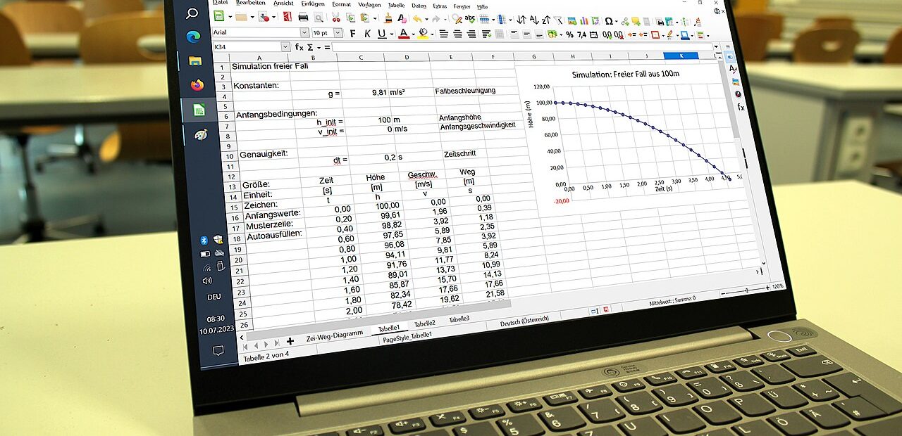
“Good knowledge of Excel” appears in job ads for accounts assistants, MIS executives, sales coordinators, HR assistants and almost every back-office role. In interviews, though, “good knowledge” usually means something specific: can you look up data from another sheet, summarise thousands of rows in minutes, stop people entering wrong values and present the result clearly? This guide covers the Advanced Excel skills that matter most for office jobs, with the exact functions, menus and shortcuts you should practise.
Which version of Excel are you using?
Some newer functions are not available in older versions, so check this first. XLOOKUP, FILTER, UNIQUE and SORT are available in Microsoft 365 and in Excel 2021 and later perpetual versions, but not in Excel 2019, 2016 or earlier. IFS is available in Excel 2019 and later and in Microsoft 365. Many offices still run older versions, so a strong candidate knows both the modern function and the older alternative, such as VLOOKUP or INDEX with MATCH.
Also learn the difference between relative references (A1), absolute references ($A$1) and mixed references ($A1 or A$1). Pressing F4 while editing a reference cycles through these. Most formula errors in offices come from copying a formula without locking the right cells.
Lookup functions: XLOOKUP and VLOOKUP
VLOOKUP
VLOOKUP searches for a value in the first column of a range and returns a value from another column in the same row:
=VLOOKUP(lookup_value, table_array, col_index_num, [range_lookup])
Example: =VLOOKUP(A2, Products!$A$2:$D$500, 3, FALSE) finds the product code in A2 on the Products sheet and returns the value from the third column. Always use FALSE (or 0) as the last argument for an exact match. Leaving it out makes Excel use an approximate match, which can quietly return wrong results.
VLOOKUP’s limits: it can only look to the right of the lookup column, and the column number breaks if someone inserts a column in the table.
XLOOKUP
XLOOKUP fixes those problems:
=XLOOKUP(lookup_value, lookup_array, return_array, [if_not_found], [match_mode], [search_mode])
Example: =XLOOKUP(A2, Products!A:A, Products!C:C, “Not found”). It can look left or right, defaults to an exact match, and lets you set a friendly message when nothing is found. In older versions, the equivalent is =INDEX(Products!C:C, MATCH(A2, Products!A:A, 0)).
Practical tip: When a lookup returns #N/A even though the value “looks” the same, the cause is usually extra spaces or numbers stored as text. Use TRIM to remove extra spaces and check the cell format, or convert text-numbers with VALUE. Fixing data before looking it up saves hours of confusion.
Logical functions: IF, IFS and friends
Logical functions let a sheet make decisions.
- IF: =IF(C2>=50000, “Target met”, “Below target”)
- Nested IF: useful in older versions for several conditions, but hard to read when there are many levels.
- IFS: checks conditions in order and returns the first match: =IFS(C2>=90, “A”, C2>=75, “B”, C2>=50, “C”, TRUE, “Fail”). The final TRUE acts as an “everything else” case.
- AND / OR: combine conditions, for example =IF(AND(C2>=50000, D2=”Delhi”), “Bonus”, “”).
- IFERROR: replaces error values with something cleaner: =IFERROR(B2/C2, 0). Use it carefully; hiding errors can hide real problems.
Conditional sums and counts: SUMIFS, COUNTIFS, AVERAGEIFS
These functions answer everyday questions such as “What were total sales in Delhi in March?” without a pivot table.
=SUMIFS(sum_range, criteria_range1, criteria1, [criteria_range2, criteria2], …)
Example: =SUMIFS(E:E, B:B, “Delhi”, C:C, “>=01-03-2026”, C:C, “<=31-03-2026”) adds the amounts in column E where the region is Delhi and the date falls in March. Dates in criteria depend on your system’s regional date format, so it is safer to put the start and end dates in cells and refer to them, for example “>=”&H1.
Note that in SUMIFS the sum range comes first, while in the older SUMIF it comes last. COUNTIFS and AVERAGEIFS follow the same pattern for counting and averaging.
Pivot tables: summarise thousands of rows in minutes
Pivot tables are the single most valuable Advanced Excel skill for MIS and reporting roles. They let you group, total and compare data by dragging fields, with no formulas.
How to build one
- Make sure your data has one header row, no blank rows or columns, and one type of data per column.
- Click anywhere in the data and press Ctrl+T to convert it into an Excel Table, so new rows are included automatically.
- Go to Insert > PivotTable and choose a new worksheet.
- Drag fields into Rows (for example, Region), Columns (Month), Values (Sum of Amount) and Filters (Product category).
- Right-click a date field and use Group to summarise by months, quarters or years.
- After adding new data, right-click the pivot table and choose Refresh.
Learn to change “Sum” to “Count” or “Average” using Value Field Settings, show values as a percentage of the total, and add slicers for clickable filters. A pivot chart built from the pivot table turns the same summary into a visual report.
Data validation and conditional formatting
Data validation
Data validation (Data > Data Validation) controls what users can type into a cell. Common uses:
- A drop-down list of departments, cities or status values, so everyone spells them the same way.
- Whole numbers between limits, such as quantities from 1 to 1,000.
- Dates within a range, for example only dates in the current financial year.
- An input message that explains what to enter, and an error alert for invalid entries.
Clean data entry makes every later lookup, SUMIFS and pivot table more reliable.
Conditional formatting
Conditional formatting (Home > Conditional Formatting) changes a cell’s look based on its value. Use it to highlight overdue dates, duplicate invoice numbers, values above or below a target, and top or bottom performers. Data bars, colour scales and icon sets make a report readable at a glance. You can also use a formula rule, such as =$F2<TODAY(), to highlight an entire row when a due date has passed.
Charts that communicate clearly
Managers rarely want to read a raw table. Choose the chart that fits your message:
| What you want to show | Suitable chart | Tip |
|---|---|---|
| Comparison between categories | Clustered column or bar chart | Sort bars from largest to smallest |
| Trend over time | Line chart | Keep dates in order on the horizontal axis |
| Parts of a whole | Pie or doughnut chart | Use only for a few categories |
| Actual vs target | Combo chart (column plus line) | Show target as a line over actual columns |
| Relationship between two numbers | Scatter chart | Label axes with units |
| Small trend inside a table | Sparklines | Good for dashboards with many rows |
Give every chart a clear title, remove unnecessary gridlines and 3D effects, and label values where they help. Pressing Alt+F1 inserts a quick default chart on the same sheet, and F11 creates one on a new chart sheet.
Power Query basics: clean data once, refresh forever
If you receive the same messy report every week, for example a bank statement, a software export or sales data from branches, Power Query can save hours. You find it under Data > Get & Transform Data (Get Data) in Excel 2016 and later and in Microsoft 365.
With Power Query you can:
- Import data from Excel files, CSV files, folders and other sources.
- Remove blank rows, unwanted columns and duplicate records.
- Split columns, trim spaces, change data types and replace values.
- Combine (append) monthly files into one table, or merge two tables like a lookup.
- Load the clean result into a sheet or straight into a pivot table.
Power Query records every step. Next month, you replace the source file and click Refresh, and all the cleaning happens again automatically. Even basic Power Query knowledge makes you stand out in interviews.
Shortcuts and habits that save time
| Shortcut | What it does |
|---|---|
| Ctrl+Arrow keys | Jump to the edge of the data region |
| Ctrl+Shift+Arrow keys | Select to the edge of the data region |
| Ctrl+T | Convert a range into an Excel Table |
| Ctrl+Shift+L | Turn filters on or off |
| Alt+= | Insert AutoSum |
| F4 (while editing a formula) | Toggle absolute and relative references |
| Ctrl+1 | Open the Format Cells dialog |
| Ctrl+; and Ctrl+Shift+; | Insert today’s date and the current time |
| Ctrl+D | Fill down from the cell above |
| Ctrl+E | Flash Fill based on a pattern you start typing |
| F2 | Edit the active cell |
Good habits matter as much as shortcuts: keep raw data on a separate sheet from reports, use Tables, name sheets clearly, avoid merged cells in data, and keep a backup before making big changes.
How to practise and prove your skills
Build two or three small projects that you can show or describe in an interview: a sales dashboard with a pivot table, slicers and charts; an attendance or fee tracker with data validation and conditional formatting; and a monthly report cleaned with Power Query. If you are an accounts candidate, practise exporting reports from Tally and analysing them in Excel, as covered in our Tally with GST guide. If you are starting from scratch, first read basic computer skills for jobs.
At NETWORK NET, Excel with lookup, logical and financial functions and pivot tables is part of the Basic Computer course, and Advanced Excel is included in the first semester of the ADCA diploma.
Key takeaways
- Know both XLOOKUP and VLOOKUP (or INDEX/MATCH), because many offices still use older Excel versions.
- IF, IFS, AND, OR and SUMIFS/COUNTIFS answer most everyday business questions.
- Pivot tables, data validation and conditional formatting are core skills for MIS and back-office roles.
- Choose charts based on the message, and keep them simple and clearly labelled.
- Power Query automates repetitive cleaning, and shortcuts plus good habits save hours every week.
Want guided practice with real office-style data? Explore the Basic Computer course or contact NETWORK NET to find a batch timing that suits you.
Frequently asked questions
What is the difference between VLOOKUP and XLOOKUP?
VLOOKUP can only return values from columns to the right of the lookup column and needs a column number, while XLOOKUP can look in any direction, uses exact match by default and lets you set a message when no match is found. XLOOKUP is available in Microsoft 365 and Excel 2021 or later.
Which Excel skills are most asked for in office job interviews?
Interviewers most often test lookups (VLOOKUP or XLOOKUP), IF and SUMIFS formulas, pivot tables, sorting and filtering, data validation, conditional formatting and basic charts. For MIS roles, Power Query and dashboards are a plus.
Is Power Query difficult to learn?
The basics are not difficult. If you can use Excel menus comfortably, you can learn to import, clean and combine data with Power Query through a few hours of guided practice, and improve with regular use.
Why does my VLOOKUP show #N/A?
Common causes are a value that genuinely does not exist, extra spaces, numbers stored as text, or a missing FALSE for exact match. Clean the data with TRIM or VALUE and make sure the lookup range is locked with absolute references.
How long does it take to learn Advanced Excel?
With regular practice, most people who already know basic Excel can become comfortable with the key Advanced Excel skills in a few weeks. Speed and confidence come from using them on real data.